Data classification with neural networks
A clear compromise between parametric and metric methods is the use of neural networks to solve classification problems. Neural networks are nonparametric models that do not require assumptions about the probability distribution of the data, but also do not use distance measures. This makes them universal classifiers that provide results even in cases where parametric and metric classifiers do not provide an acceptable solution.
Classification is one of the most important tasks of data mining. It is solved with the help of analytical models called classifiers. The demand for classification is due to the relative ease of application of algorithms and methods, as well as the high interpretability of the results compared to other data analysis techniques.
Currently, a large number of different types of classifiers have been developed, for the construction of which both statistical methods (logistic regression, discriminant analysis) and machine learning methods (neural networks, decision trees, k-nearest neighbors method, support vector machines, etc.) are used.
The need to use a large number of different classification methods in data analysis arises from the fact that the problems to be solved with their help may have their own specific characteristics related, for example, to the number of classes (binary classification or with multiple classes) or to the representation of the original data - its scale, dimensionality and quality - which requires the selection of an appropriate classifier. Therefore, the choice of a classifier that matches the characteristics of the analysis problem to be solved is an important factor for a correct solution.
The different types of classifiers have advantages and disadvantages. For example, classifiers that use statistical methods have good mathematical validity, but are difficult to use and require knowledge of the probability distribution of the raw data and estimation of its parameters (hence they are called parametric), as well as a fixed model structure. Moreover, statistical methods only estimate the probability of an object belonging to a class, but they do not "explain" why.
Classifiers based on machine learning do not require estimation of the parameters of the distribution of the raw data, and their similarity measure is formalized by a distance function (usually Euclidean). Such classifiers are called metric classifiers. They are usually easier to implement and use than parametric methods, and their results are easier to interpret and understand. At the same time, metric classifiers are also heuristic models - they provide a solution only in a limited number of practically significant cases and may provide an inaccurate solution or not the only solution. Therefore, their results must be used with some caution.
A certain compromise between parametric and metric methods is the use of neural networks to solve classification problems. Namely, NS are nonparametric models that do not require assumptions about the probability distribution of the data, but also do not use distance measures. This makes them universal classifiers that provide results even in cases where parametric and metric classifiers do not provide an acceptable solution.
Characteristics of using neural networks as classifiers
It should be noted that the classification problem is generally not the main problem for neural networks (as it is for decision trees or k-nearest-neighbor algorithms). Originally, the main goal of neural networks is numerical prediction (where the input and output of the model are numerical values, sometimes incorrectly called regression).
However, using special data representation methods, it is possible to adapt neural networks to handle categorical data, i.e., to obtain categorical values as input and to produce categorical values as output. For this purpose, categorical attributes are appropriately encoded with numeric values.
However, the use of neural networks as classifiers has a number of advantages that can be highlighted:
- Neural networks are self-learning models that require little or no user intervention;
- Neural networks are universal approximators that can be used to approximate any continuous function with acceptable accuracy;
- Neural networks are nonlinear models that allow effective solution of classification problems even in the absence of linear separability of classes (see figure below).

It should be noted that there are no specific neural network architectures for classification. The most commonly used network architecture for classification is the forward propagation network, which reads the feature values of the object to be classified and outputs a label or numeric class code. Usually, multilayer perseptrons are used. In such networks, the elements of a feature vector arrive at the input neurons and are distributed to all neurons in the first hidden layer of the neural network, changing the dimensionality of the problem.
Subsequent layers therefore divide objects into classes in the feature space with a higher dimensionality than the original space. For example, if the dimensionality of the feature vector of the original data is four and the hidden layer contains six neurons, then the output layer divides the features into classes in six-dimensional space.
This increases the efficiency of the process: the proper choice of the neural network configuration and parameters makes it possible to obtain good classification results even if the classifiers of other types, working only in the dimensionality of the training data, do not provide acceptable results. The drawback is that the network configuration that best approximates the class separation function in feature space is not known in advance. Therefore, it must be selected experimentally or experience with similar solutions must be used.
If the distribution of classes is such that a complex function is required to partition them, the dimensionality of neural networks may be unacceptably large. In this case, the problem can be solved by special preprocessing of the input data.
Preparation of the source data
No matter how advanced the methods and algorithms used for classification are, they will not provide correct results if applied to unclean data. Therefore, the first step in building a neural network-based classification model is to preprocess and clean the data.
The first step in this direction is to select features that are useful for distinguishing classes. Indeed, objects in a domain can be described by a large number of features. But not all of them can reliably distinguish between objects of different classes. For example, if objects of different classes have approximately the same size, it makes no sense to use "dimensional" features. It is also not desirable to use features whose values are random and do not reflect patterns in the distribution of objects between classes.
In addition, it is important to determine the number of features used. The more features used to create a classifier, the more information is used to distinguish classes. However, this increases the computational cost and the requirements for the size of the neural network (the number of parameters that can be adjusted in the learning process - weights of neuron connections). On the other hand, reducing the number of features used worsens the separability of the classes. For example, it may happen that objects of different classes have the same meaning of features and a contradiction arises.
For example, only two characteristics can be selected for classifying borrowers as "bad" and "good": "income" and "age". It is likely that two borrowers of the same age and income would fall into different classes. Another attribute, such as the number of dependents, should be added to distinguish borrowers. Therefore, selecting features for training a classifier based on a neural network is a compromise solution.
Another important method for preprocessing the training data is to normalize the attribute values to a range of 0...1. Normalization is necessary because the classification attributes are of different physical nature and their values may differ by several orders of magnitude (e.g., "income" and "age").
In addition, before creating a neural network-based classifier, a data profile should be created to assess data quality and, if necessary, data cleaning tools should be used: Fill gaps, suppress anomalous values and outliers, exclude duplicates and inconsistencies.
Coding of the output values
The fundamental difference between the classification problem and the numerical prediction problem is that the output variable is discrete (the class label or its numerical code). Since neural networks are supervised learning models, the class variable must be specified for each training example.
In the simplest case, when the classification is binary, the problem can be solved by a neural network with a single output layer neuron that outputs two possible states (for example, 0 and 1). If there are multiple classes, the problem of their representation in the output of the network must be solved. In practice, the output vector is usually used, whose elements are labels or class numbers.
In this case, the membership of an object to a class is determined by setting the corresponding element of the output vector (the i-th element for the j-th class) to 1, while the other elements are set to 0. Then, for example, the second class at the second output of the network corresponds to a 1 and to 0 at the others.
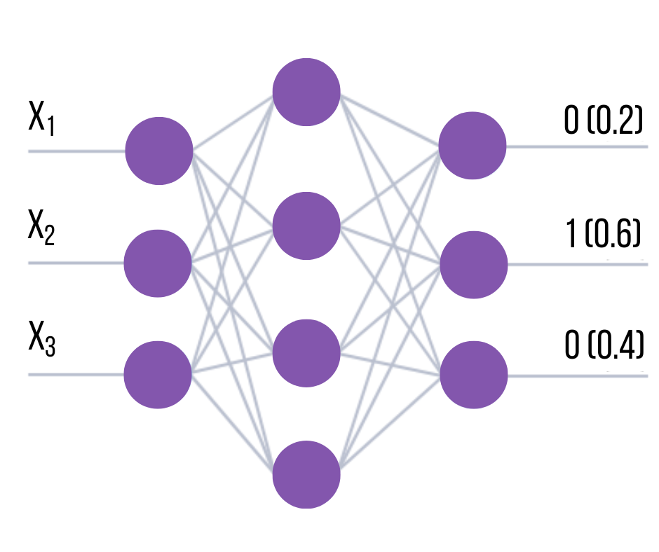
Values other than 1 can also be used for coding. However, when interpreting the result, it is usually assumed that the class is determined by the number of the network output where the highest value occurred. For example, if a vector of output values (0.2, 0.6, 0.4) was generated at the output of the network, the second component of the vector would have the highest value. Consequently, the class referred to in this example would be 2.
With this type of encoding, the more different the maximum value is from the others, the more certain it is that the net has assigned the object to the class. Formally, this confidence can be entered as an index equal to the difference between the maximum value at the input of the network (which determines class membership) and the closest value at the other output.
For the above example, the confidence of the network that the example belongs to the second class is determined as the difference between the second and third components of the vector and is equal to 0.6-0.4=0.2. The higher the confidence, the higher the probability that the network gave the correct answer. This coding method is the simplest, but not always the most efficient way of representing classes in the output of the network.
For example, in another representation method, the class number is encoded in binary form in the output vector of the net. If the number of classes is 5, three output neurons are sufficient to represent them, and the code corresponding to, for example, the third class is 011. The disadvantage of this approach is the lack of possibility to use the confidence index, since the difference between any elements of the output vector always equals 0 or 1. Consequently, the change of any element of the output vector inevitably leads to an error. Therefore, it makes sense to use the Hamming code to increase the "distance" between classes, which increases the classification accuracy.
Another approach is to split the problem with k classes into k∗(k-1)/2 subtasks with two classes each (2-by-2 coding). In this case, the subtask is for the network to determine the presence of a component of the vector. In other words, the output vector is divided into groups of two components each, so that all possible combinations of the components of the output vector are included in these groups. It is known from combinatorics that the number of these groups can be defined as the number of unordered samples without repetitions of two of the original components:
For example, for a task with four classes, there are six outputs (subtasks) distributed as follows:
| Subtask (Output) | Classes |
|---|---|
| 1 | 1-2 |
| 2 | 1-3 |
| 3 | 1-4 |
| 4 | 2-3 |
| 5 | 2-4 |
| 6 | 3-4 |
Here, a 1 in the output indicates the presence of one of the components. Then the class number is determined from the result of the network calculation as follows: Determine which combinations received a single (or approximate) output value (i.e., which subtasks were activated), and assume that the class number should be the one that was included in the largest number of activated subtasks (see table).
| Class | Subtasks (Outputs) |
|---|---|
| 1 | 1, 2, 3 |
| 2 | 1, 4, 5 |
| 3 | 2, 4, 6 |
| 4 | 3, 5, 6 |
This coding method provides better classification results than classical approaches for many tasks.
Selection of the network size
To create an efficiently functioning classifier, it is very important to choose the right size of the network, i.e., the number of connections between the neurons that will be established in the learning process and will process the input data when the process is running. If the number of weights in the network is small, it cannot implement complex class separation functions. On the other hand, more links leads to an increase in the information capacity of the model (weights act as memory elements).
If the number of links in the network exceeds the number of training examples, the network will not approximate the dependencies in the data, but will simply remember and reproduce the input-output combinations from the training examples. This classifier will work well with the training data and produce arbitrary responses for the new data that was not included in the training process. In other words, the network will not gain generalization ability, and the classifier built on its basis will be useless in practice.
There are two approaches, one constructive and one destructive, to right-sizing the network. The first is to first take a minimal size network, which is then gradually increased until the required accuracy is achieved. After each increase, it is re-trained. There is also the so-called cascade correlation method, where the network architecture is adjusted after each training epoch to minimize the error.
In the destructive approach, we first take an oversized network and then remove the neurons and connections that have the least impact on the accuracy of the classifier. It is useful to remember the following rule: the number of examples in the training set must be larger than the number of tunable weights of the network. Otherwise, the network will not be able to generalize and will produce arbitrary values for the new data.
To test the generalization ability of the network on which the classifier is built, it is useful to use a test set formed from randomly selected examples of the training data set. The examples of the test set do not participate in the training process of the network (i.e., they do not affect the adjustment of its weights), but are simply fed into the input of the network together with the training examples.
If the network has high accuracy on both the training set and the test set (whose examples play the role of the new data), the network can be said to have achieved generalization capability. If a network only performs well on the training data and poorly on the test data, it is not capable of generalization.
The network error is often referred to as the training error in the training set and the generalization error in the test set. The ratio of training and test sets can be arbitrarily large. The test set must contain enough examples for the model to be properly trained.
The obvious way to improve the generalization ability of the network is to increase the number of training examples or decrease the number of connections. The former is not always possible due to the limited amount of data and increased computational effort. Reducing the number of connections, on the other hand, affects the accuracy of the network. Therefore, the choice of model size is often quite complex and requires repeated trials.
Selection of the network architecture
As mentioned earlier, no special neural network architectures are used to solve the classification problem. The typical solution for this is flat networks with sequential connections (perseptrons). Usually, several network configurations with different number of neurons and their organization in layers are tested.
In this case, the main indicator for a choice is the size of the training set and the achievement of the generalization capability of the network. Commonly, a backpropagation learning algorithm with a validation set is used.
Algorithm for building a classifier
Building a neural network based classifier involves a series of steps.
-
Preparation of the data
- Creation of a database with examples that are typical for the task
- Division of the entire Data set into two sets: Training and Test (a division into 3 sets is possible: Training, Test and Validation).
-
Preprocessing of the data
- Selection of features relevant to the classification task.
- Transformation and, if necessary, cleaning of the data (normalization, removal of duplicates and inconsistencies, removal of outliers, etc.). As a result, it is desirable to obtain a space of example sentences linearly separated by class.
- Selection of the output coding system
-
Design, training and quality assessment of the network
- Selection of the network topology: number of layers, number of neurons in the layers, etc.
- Selection of the activation function of the neurons (e.g. logistic, hypertangential, etc.)
- Selection of the learning algorithm
- Estimation of the network performance based on the validation set or other criteria to optimize the architecture (reduction of weights, thinning of the feature space)
- Deciding on the version of the network that provides the best generalization capability and evaluating the quality of the performance on the test set
-
Usage and diagnosis
- Finding out to what extent different factors influence the decision (heuristic approach).
- Verify that the network achieves the required classification accuracy (the number of misrecognized examples is small)
- If necessary, go back to step 2 and change the way the examples are presented or change the database
- Practical use of the network to solve the problem.
To create an effective classifier, the input data must be of good quality. No classification method based on neural networks or statistical methods will ever provide the desired model quality if the available set of examples is not sufficiently complete and representative of the problem being solved.